Snowflake Query Optimization: 7 Tips for Faster Queries
Slow queries have been the bane of humanity for as long as databases have existed. In Snowflake, a small optimization in a SQL query can often lead to dramatically faster queries.
Snowflake Query Bottlenecks
Before learning how to optimize a query we first have to understand what causes slow queries in Snowflake. Bottlenecks broadly fall into three categories-
1. Reading more data than necessary
Imagine you had to figure out when Harry Potter first goes to Hogwarts. You're given two options: read the entire eight-book series or only read the first book. The latter will be much faster. The same applies to databases - the less data there is to read, the faster the query will be.
In Snowflake terms, this process is known as a table scan. It involves reading data from Snowflake's storage layer into the compute layer. The more data scanned, the slower and more expensive your query becomes.
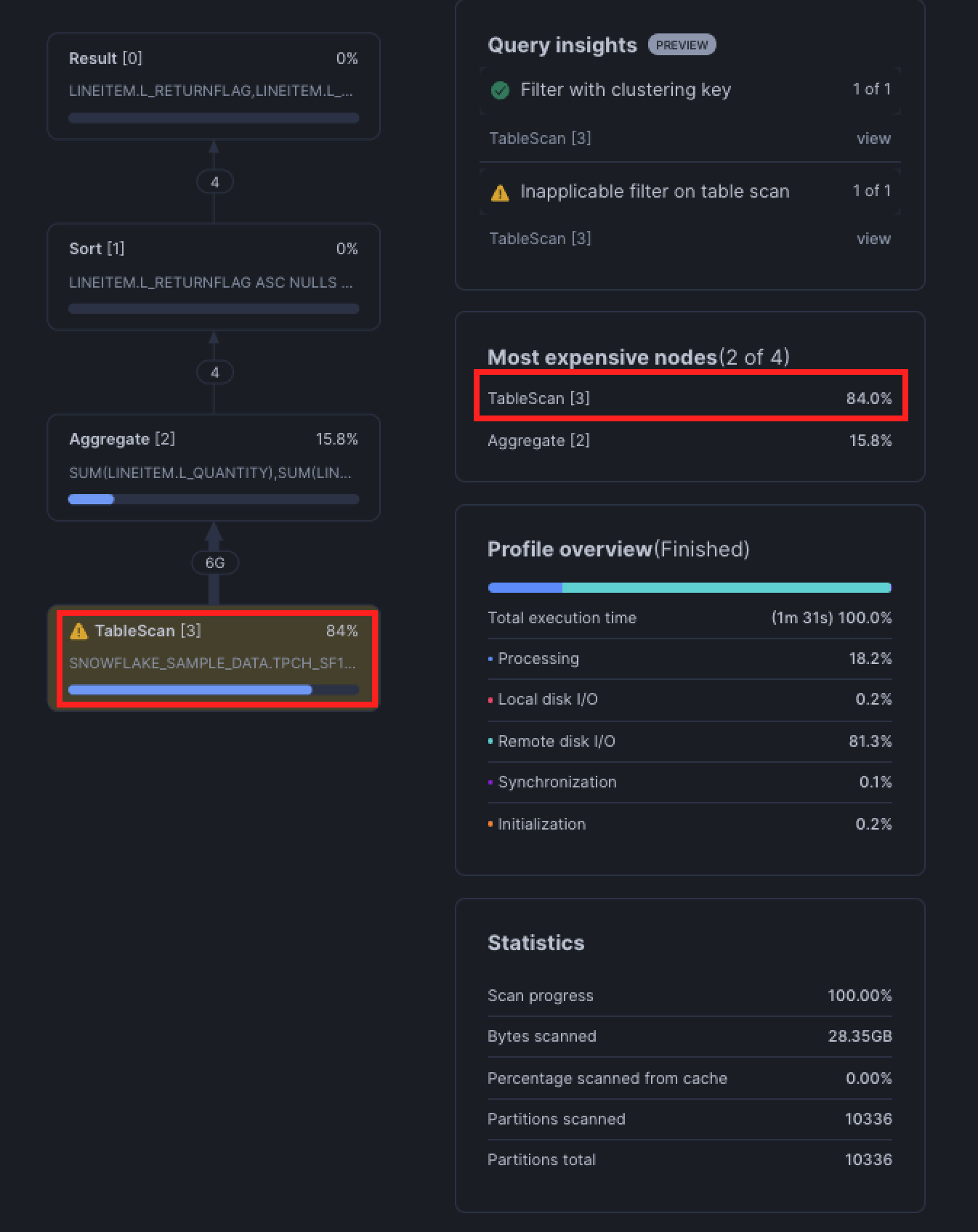
The key here is to reduce the amount of data read in our TableScan node in the query plan. Efficient queries minimize the amount of data scanned by:
- Leveraging Snowflake's micro-partition pruning capabilities and caching
- Using appropriate filters in the WHERE clause and placing them as early as possible
- Selecting only necessary columns instead of using SELECT *
2. Functions That Operate On or Create a Lot of Data
Once data is read into the compute layer, Snowflake needs to process it according to the query's instructions. This can involve various operations that can be computationally expensive:
- Joins: Combining data from multiple tables, especially for large datasets or complex join conditions. Joins that create more records than originally input (many-to-many) can cause significant reduction in query performance.
- Aggregations: GROUP BY operations, particularly on high-cardinality columns, can require significant processing power.
- Sorting: ORDER BY operations on large result sets can be resource-intensive.
Complex queries that involve multiple of these operations can lead to even longer execution times and high resource utilization.
3. Virtual Warehouse Misconfigured
Sometimes, the warehouse is either not setup properly or the query itself requires a larger warehouse. The most obvious sign that your warehouse is too small is if queries are spilling to local or remote storage.
Spilling happens when Snowflake warehouse runs out of memory. Data is first spilled (in other words, written) to the local SSD, and if that runs out of memory, it is spilled to remote storage. Because spilling adds extra I/O operations, these queries will always run slower than those that full fit into memory.
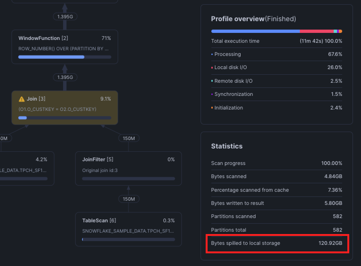
Spilling is essentially Snowflake’s safety net: your query will still complete, but performance can degrade dramatically. If you see local spills, it’s a yellow flag—there may be room to optimize filters, aggregations, or data pruning. Remote spills are a red flag that either the query is creating oversized intermediates, or your warehouse is under-provisioned.
Before you decide to upsize your warehouse, see if there is a way to tune your query to reduce the amount of data being processed: improving partition pruning, projecting only the required columns, or split the processing into several steps.
Optimization Techniques
Before we begin optimizing a query, we first need to understand where it's slow. Luckily for Snowflake users, we've been equipped with the query profile, a detailed breakdown of how Snowflake executes your query.
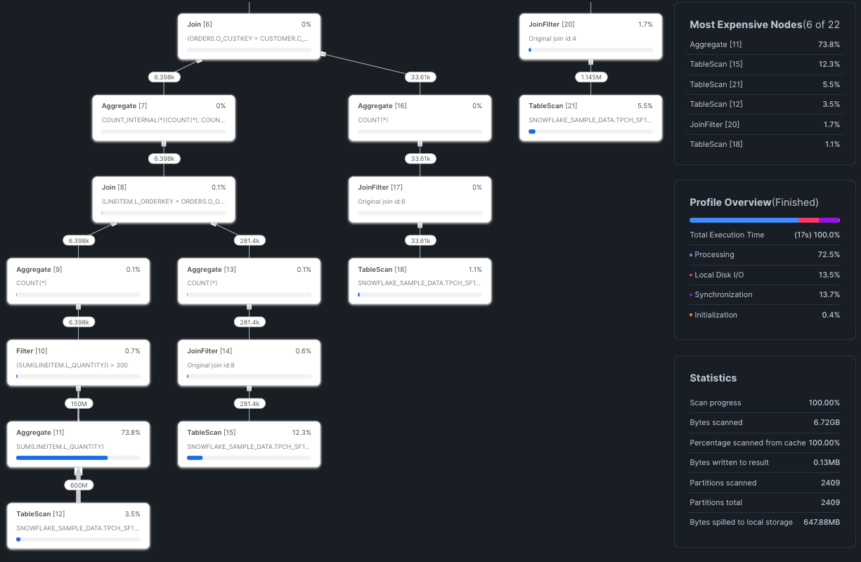
Reviewing the Most Expensive Nodes section, we see that Snowflake spent 74% of the time on an Aggregate operation in node 11. This is where we would want to focus our optimization.
1. Reduce Amount of Data Read (Query Pruning)
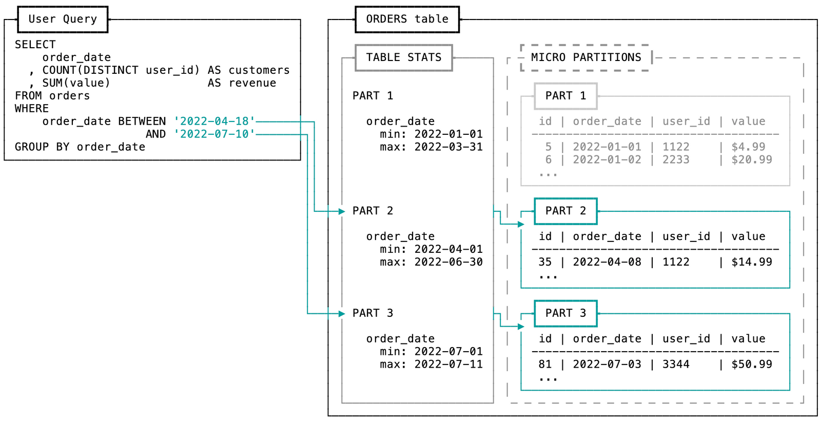
Snowflake uses predicate pushdown through query pruning. Filters in your WHERE clause are pushed down and applied at the storage layer so that Snowflake can read less data into memory. In other words, Snowflake only reads the data that is necessary to execute your query, instead of reading an entire dataset and then filtering it in memory.
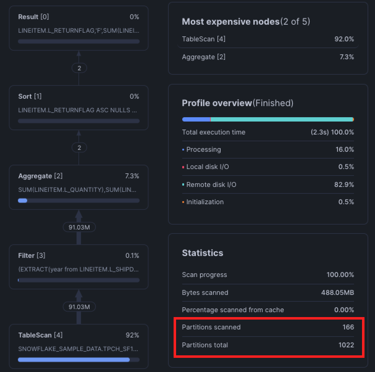
To determine whether your query is pruning, review the query's Partitions Scanned against the Partitions Total in the bottom right Statistics tile. If a query is pruning properly, the Partitions Scanned will be less than the Partitions Total.
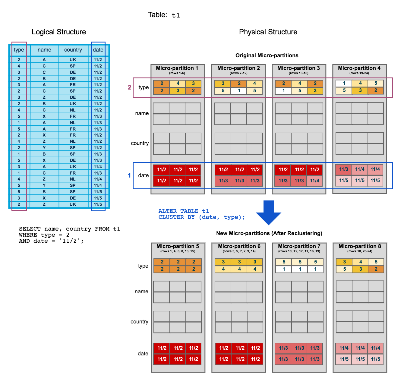
In practice, however, pruning doesn't always work. Pruning is only effective when the columns you filter on are clustered within Snowflake's micro-partitions (micro-partitions are how Snowflake stores and organizes data). Columns that tend to have a natural sort order like dates or ones with low cardinality like region often become clustering keys.
Typically, data stored in tables is sorted/ordered along natural dimensions (e.g. date and/or geographic regions). These ordered columns are "clustering keys".
As data is inserted/loaded into a table, clustering metadata is collected and recorded for each micro-partition created during the process. Snowflake then leverages this clustering information to avoid unnecessary scanning of micro-partitions during querying, significantly accelerating the performance of queries that reference these columns.
More on this in section 6!
How to Query Prune
Write simple and direct filters in your WHERE clause! Try your best to apply filters as early as possible. Most of the time, query pruning will just work, but it can fail from:
- Functions or complex expressions in the
WHEREclause - Type conversions in the
WHEREclause. Converting timestamps to dates will still allow pruning to work - Filtering on a column that's not clustered. Tables can become less clustered over time.
- Filtering on certain JSON fields, depends on the data in your JSONs
Query pruning is one of the most effective Snowflake query optimization techniques for reducing both cost and runtime.
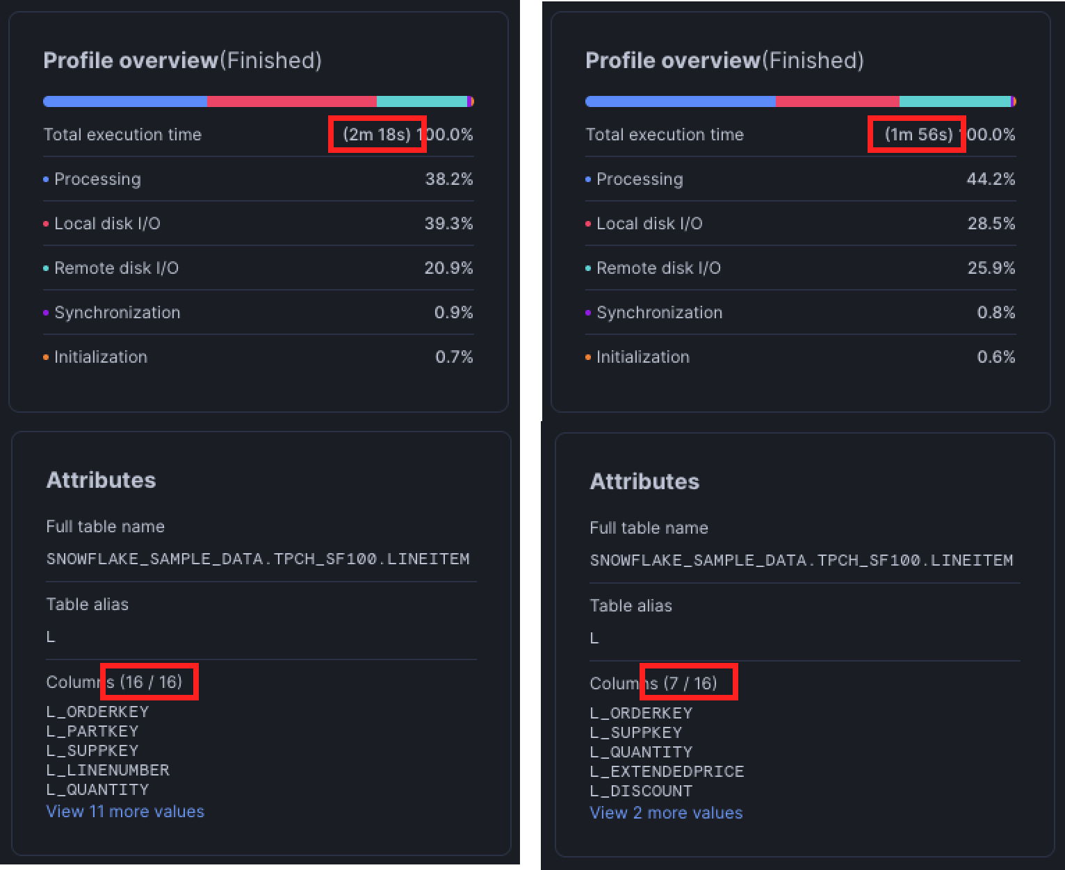
2. Avoid SELECT *
In other words, only select the columns you actually need. Snowflake’s optimizer is smart—it's able to column prune, which means that if your query doesn’t use certain columns, they won’t even be read from storage.
For example, even though the CTE below uses a SELECT *, the final query only references c_name and filters on c_mktsegment, so the table scan only fetches those two columns.
WITH customers AS (
    SELECT
        *
    FROM snowflake_sample_data.tpch_sf100.customer
)

SELECT
    c_name AS customer_name
FROM customers
WHERE
    c_mktsegment = 'AUTOMOBILE';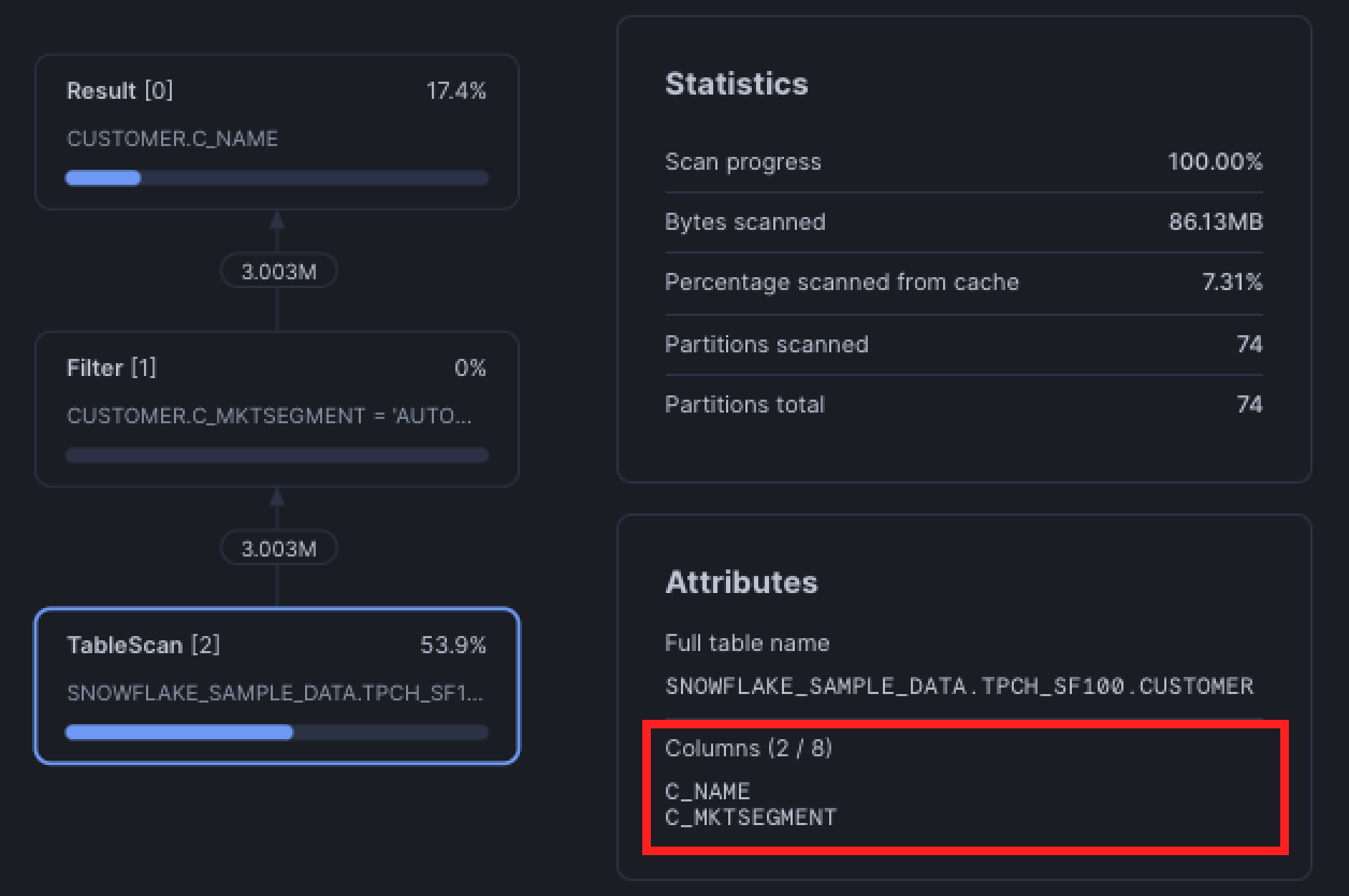
But if you finish the query with another SELECT *, Snowflake has no choice but to fetch every column, whether you need them or not. Snowflake's optimizer can prune unused columns, but it can't magically drop columns if the final query explicitly asks for them.
WITH customers AS (
    SELECT
        *
    FROM snowflake_sample_data.tpch_sf100.customer
)

SELECT
    *
FROM customers
WHERE
    c_mktsegment = 'AUTOMOBILE';
You shouldn’t assume Snowflake’s optimizer will always handle column pruning correctly. When pruning fails, the performance difference can be dramatic: tens of seconds on small tables, and up to 10x slower queries when working with wide tables (hundreds of columns) and billions of rows.
The query we used to demonstrate this is fairly large, so you can find the full version in the appendix at the end of this post.
3. Optimize Joins
Joins are often a major bottleneck in queries as there are many common pitfalls that can cause a join to be terribly slow.
Avoid using OR
Observe the query below.
SELECT
    l_orderkey
    , l_partkey
    , l_suppkey
    , l_quantity
FROM snowflake_sample_data.tpch_sf1.lineitem AS l
JOIN snowflake_sample_data.tpch_sf1.partsupp AS p
    ON l.l_partkey = p.ps_partkey
    OR l.l_suppkey = p.ps_suppkey;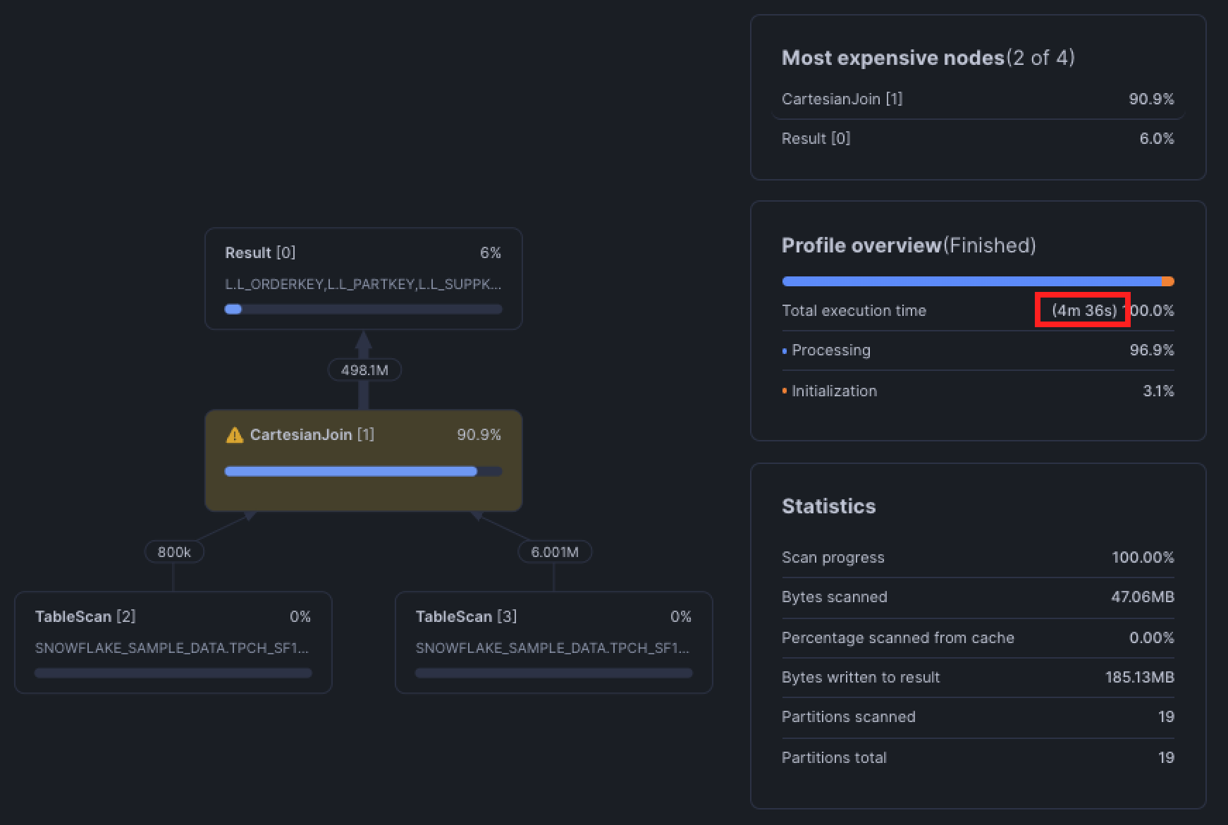
This is known as a disjunctive join, a join condition that uses OR between two or more predicates.
The problem is that query optimizers, including Snowflake's, are optimized for equi-joins (a single condition like id = id) as the fast path. With a direct equi-join, Snowflake can partition and hash efficiently, push down filters, and prune.
But when you use OR in the join condition Snowflake no longer has one clear key to partition on, it has to account for matches on either column. Pruning and join filters break down because the engine can't confidently eliminate partitions based on one column alone.
Taking a look at the query profile, Snowflake falls back to a Cartesian join, meaning it's generating all possible row combinations between the two tables and then applying the OR condition afterwards to filter. You'll notice that this happens in the range join pitfall in the next section.
Fix it with UNION ALL
The easiest way around the OR is to split the query into two equi-joins and then stitch the results together with a UNION ALL.
SELECT
    l_orderkey
    , l_partkey
    , l_suppkey
    , l_quantity
FROM snowflake_sample_data.tpch_sf1.lineitem AS l
JOIN snowflake_sample_data.tpch_sf1.partsupp AS p
    ON l.l_partkey = p.ps_partkey

UNION ALL

SELECT
    l_orderkey
    , l_partkey
    , l_suppkey
    , l_quantity
FROM snowflake_sample_data.tpch_sf1.lineitem AS l
JOIN snowflake_sample_data.tpch_sf1.partsupp AS p
    ON l.l_suppkey = p.ps_suppkey;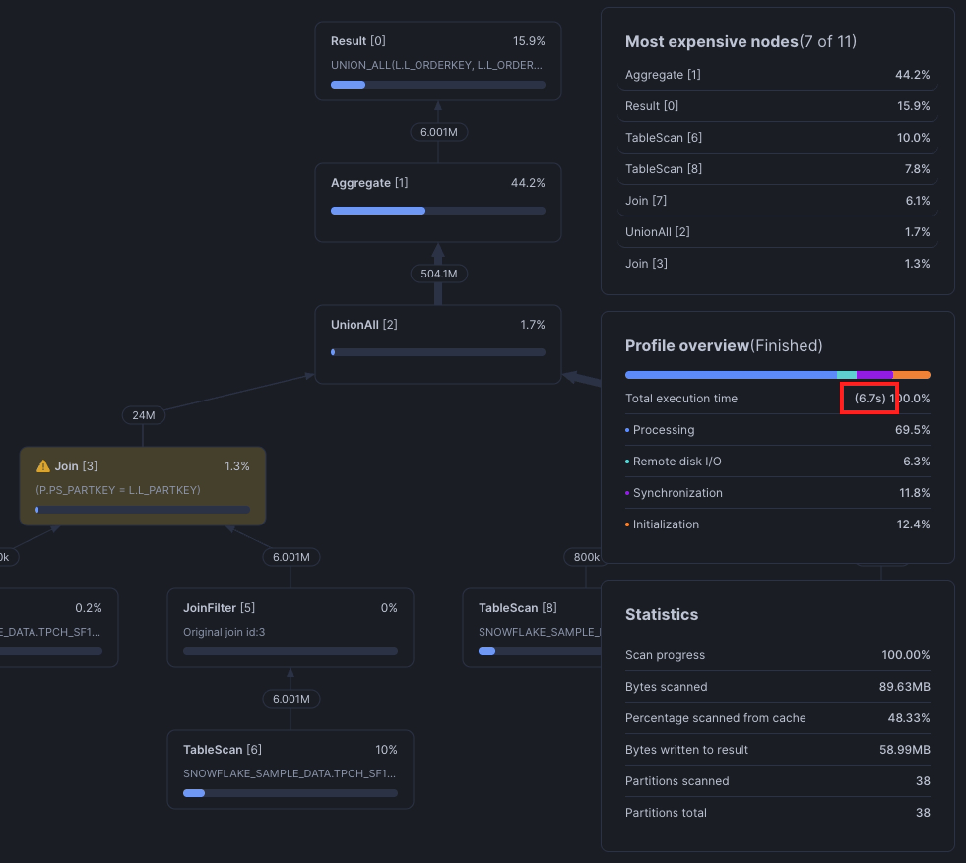
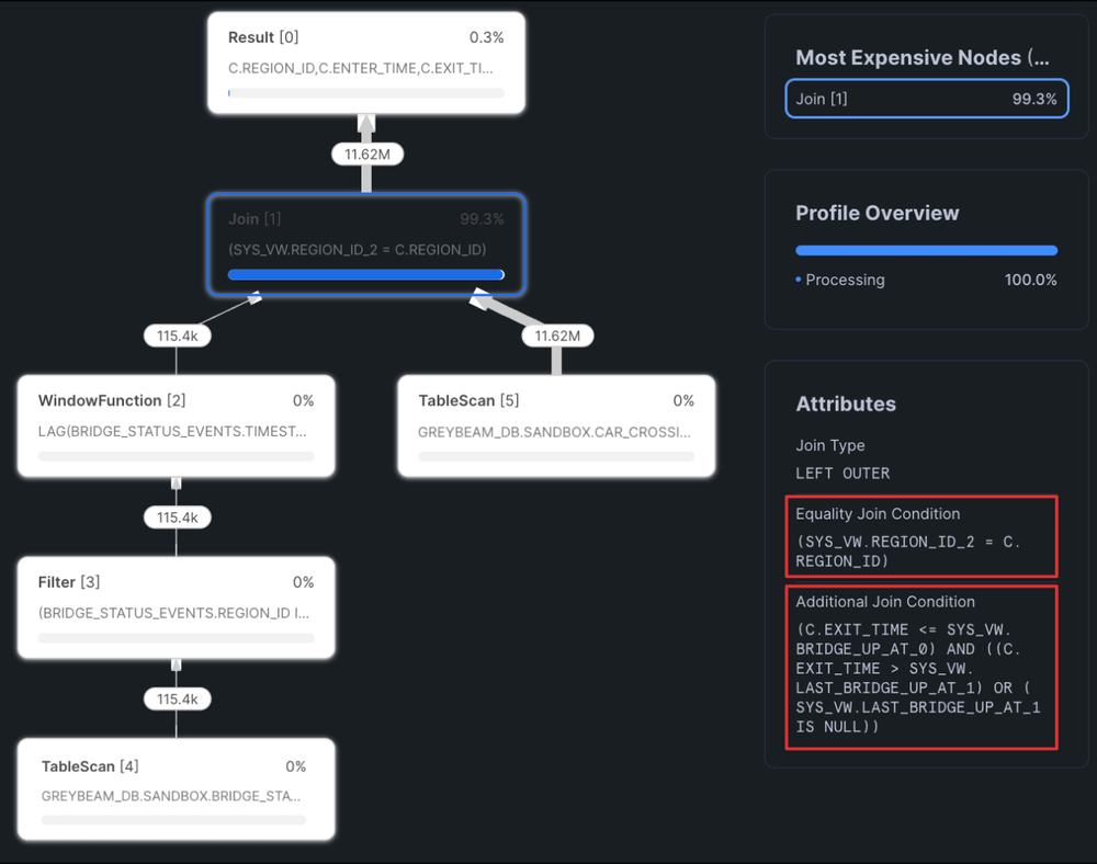
Optimize Range Interval Joins
As previously discussed, most query optimizers excel at equi-joins. However, we often find the need to join records that fall within a range values, for example, what was the price of gasoline for each refill at the gas station? You would need to determine which price was valid during each refill. In practice, this means joining the refill timestamp against the valid_from and valid_to columns in the gas prices table. It might look something like this.
SELECT
r.refill_id,
r.refill_time,
p.price
FROM refills r
JOIN gas_prices p
ON r.refill_time >= p.valid_from
AND r.refill_time < p.valid_to
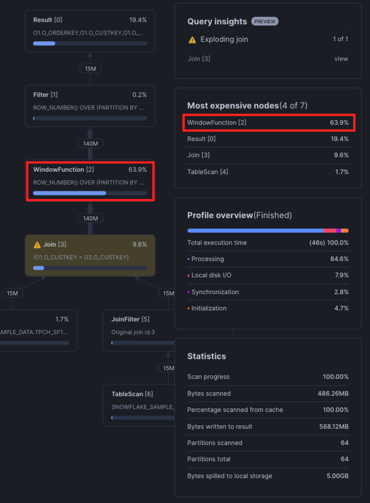
AND r.gas_station_id = p.gas_station_id;These are range joins and are typically seen when using join operators such as BETWEEN, <, <=, >, or >=. Similar to the disjunctive join above, Snowflake tends to use a Cartesian join between the two tables and then applying the range join condition after. A Cartesian join between two tables with 10,000 records will generate an intermediate dataset with 100 million records! You can see how quickly this explodes and slows down query performance as the query generates intermediate data and spills to disk and/or remote storage.
Fix with an ASOF
ASOF joins are handy when you need to find a record in the right table that is closest in time to the left table. You can quite literally read ASOF as "as of", as in, as of this time which record is the closest? We cover ASOF joins in-depth in a previous article.
SELECT
    r.refill_id,
    r.refill_time,
    p.price
FROM refills r
ASOF JOIN gas_prices p
  MATCH_CONDITION (r.refill_time >= p.valid_from)
  ON r.gas_station_id = p.gas_station_id;
In this case, the ASOF join will join the closest record in time from gas_prices that is less than the refill time.
Fix with Binning
We won’t be getting into the details of binning in this blog, but the concept is straightforward. As we’ve discussed, Snowflake performs a Cartesian join between the tables, but this join can be limited by any additional equi-join conditions. To reduce the number of comparisons Snowflake has to make, we can introduce more equi-joins. One simple way to do this is by restricting the join on a time-based bin (for example, grouping by day, hour, or another fixed interval).
SELECT
    r.refill_id,
    r.refill_time,
    p.price
FROM refills r
JOIN gas_prices p
  ON r.refill_time >= p.valid_from
  AND r.refill_time <  p.valid_to
  AND DATE_TRUNC('DAY', r.refill_time) = DATE_TRUNC('DAY', p.valid_to)
  AND r.gas_station_id = p.gas_station_id;
Binning can get fairly complex and there is a brilliant example from our friends at Select that you can find here.
Joining on Cluster Keys
When tables are frequently joined on a common set of keys, such as id or date, you can improve join performance by clustering on those keys.
A clustering key is a subset of columns Snowflake uses to physically organize data in its storage layer. Similar to pruning (from the previous section), clustering helps Snowflake skip over large portions of data that don’t match your query filters, rather than scanning the entire table. For example, if our orders table is clustered by order_date, Snowflake can completely ignore data older than 7 days.
SELECT
   *
FROM orders
WHERE
   order_date > current_date - 7;
Keep in mind that creating and maintaining clustering keys consumes credits. Always evaluate whether clustering is actually improving performance, and consider removing it if it isn’t. You can check clustering effectiveness with:SELECT SYSTEM$CLUSTERING_INFORMATION('MY_DB.MY_SCHEMA.MY_TABLE');
Creating a table with cluster keys:
CREATE OR REPLACE TABLE orders AS
   SELECT * FROM orders
CLUSTER BY (order_date);
Adding cluster keys to an existing table:
ALTER TABLE orders CLUSTER BY (order_date);In dbt:
{{
  config(
    materialized='table',
    cluster_by=['order_date']
  )
}}

select
  id::varchar as order_id
  , order_date::date as order_date
  , order_price::number as order_price
from {{ source('prod', 'orders') }}
This can be useful particularly in dbt jobs with slow incremental builds. When using an incremental strategy in dbt, either a MERGE or DELETE+INSERT will be executed under the hood. These typically involve full table scans on the unique key specified. You can, however, specify incremental predicates, and if the incremental predicates are set on clustered columns then your incremental build can skip performing a full table scan.
{{
  config(
    materialized = 'incremental',
    unique_key = 'id',
    cluster_by = ['order_date'],
    incremental_strategy = 'merge',
    incremental_predicates = [
      "DBT_INTERNAL_DEST.order_date > dateadd(day, -7, current_date)"
    ]
  )
}}
Forcing a Join Order
Snowflake uses hash joins to build its joins. This means the left table is used to build a hash table, then the right table probes the hash table to find matches. The left table is known as the Build side and the right is the Probe side.

The build side requires more memory, so when the larger table is used as the build side, query performance can degrade, especially if memory spills!
Most of the time however, Snowflake's optimizer will build the query plan properly. But what if it doesn't?
Directed Joins
Force join orders using a directed join! The table that is DIRECTED will be used as the probe (right) side. Observe the example below:
SELECT
    *
FROM snowflake_sample_data.tpch_sf10.orders AS o
JOIN snowflake_sample_data.tpch_sf10.lineitem AS l
    ON o.o_orderkey = l.l_orderkey
WHERE
    LEFT(l.l_shipmode, 1) = 'A'
;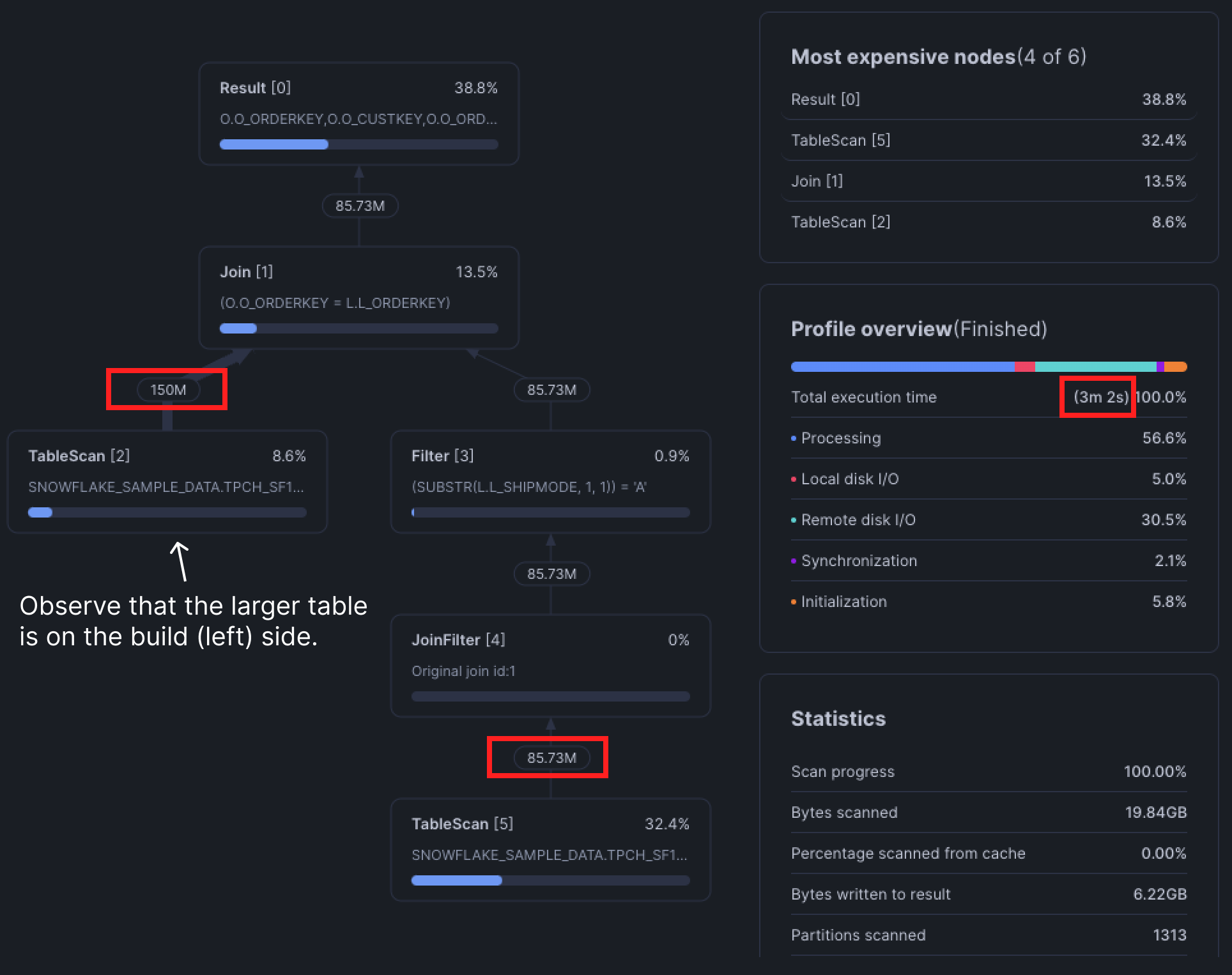
Now let's see what happens when we flip the joins by adding DIRECTED to the second join clause.
SELECT
    *
FROM snowflake_sample_data.tpch_sf100.lineitem AS l
INNER DIRECTED JOIN snowflake_sample_data.tpch_sf100.orders AS o -- forces Snowflake to use this table on the probe (right) side
    ON o.o_orderkey = l.l_orderkey
WHERE
    LEFT(l.l_shipmode, 1) = 'A'
;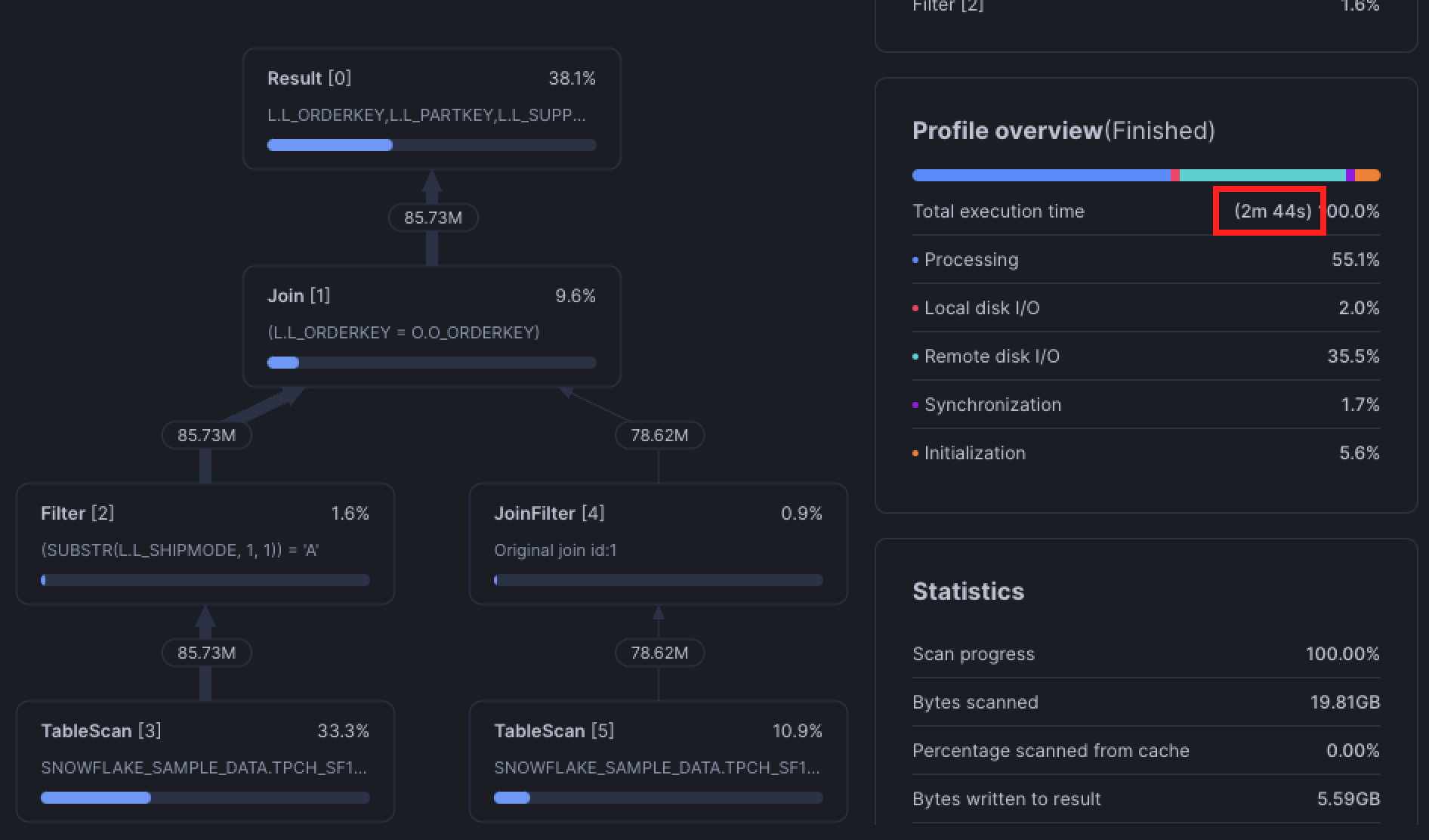
You can use the DIRECTED keyword with any join!
Similar to clustering, this optimization will have a more significant effect when there is more data involved.
4. Complex Views
Views are handy for encapsulating light business logic and keeping the queried data in-sync with upstream data, but views can hide much complexity in plain sight. Every time you query a view, Snowflake executes its underlying SQL. If that view references another view, which references another view, and so on, the final query plan can balloon into something far larger and more complex than you expect.
The simple solution is to split the view into smaller parts and persist them as tables. However, if your business requires the data to be real-time, you may need to understand whether that means seconds, minutes, or hours delayed. Chances are they don't actually need real-time data.
5. Proper Use of Warehouse Cache
Proper usage of warehouse cache is the most simple but overlooked Snowflake optimization technique.
Whenever Snowflake executes a query, data is pulled from remote storage and staged in the virtual warehouse's local SSDs. Subsequent queries that retrieve data from the same tables can reuse that cached data as long as they're running on the same warehouse.
As a rule of thumb, keep related workloads–especially those that query similar tables–on the same warehouse so they can take advantage of this shared cache. Consolidating workloads has an added benefit of reducing costs, as warehouses are typically underutilized. Just remember that the warehouse cache is cleared whenever a warehouse suspends, so choosing an appropriate AUTO_SUSPEND is key to balancing cost savings and cache usage.
6. Clustering
Clustering is Snowflake's way of organizing data so that related records are physically close together in storage. In practice, this means a clustering key is used to co-locate similar rows within the same micro-partitions, making query pruning far more likely.
By default, clustering in Snowflake happens organically: data is written to micro-partitions in the order it arrives. This means you could naturally cluster data by asserting an ORDER BY at the end of your CREATE TABLE AS SELECT. However, if your tables are built incrementally, the natural order of the table can get messy as new data arrives, making query pruning less effective.
Benefits from clustering are generally more pronounced on very large tables (think billions of records or multiple terabytes of data). On smaller tables, scanning a few extra partitions isn't a big deal. But at scale, poor clustering can be the difference between scanning 5% of a table vs 100% of it. Benefits include:
- Faster queries via improved scan efficiency by skipping over data that don't match filter predicates (pruning!)
- Better column compression, especially when other columns are strongly correlated with the columns that comprise the clustering key
When to Consider Clustering
Clustering is best for a table that generally meets all of the following criteria:
- The table is at least multiple terabytes or larger.
- Queries on this table are often selective. In other words, queries only read a small percentage of rows, for example, last 7 days of data or a specific customer.
- Queries that join to this table frequently join on similar clustering keys.
Before deciding whether you should cluster a table, please consider the associated credit and storage costs alongside testing a representative set of queries on the table to establish performance baselines. We will get into this in a future blog.
How to Cluster Tables
There are a few ways to cluster a table, the first is during creation:
-- Explicitly clustering by columns
CREATE OR REPLACE TABLE orders (id STRING, customer_id, STRING, order_date DATE, price NUMBER)
   CLUSTER BY (customer_id, order_date);

-- Natural clustering with an ORDER BY
CREATE OR REPLACE TABLE orders AS
   SELECT * FROM orders_raw ORDER BY customer_id, order_date DESC;
Adding or change a clustering key of an existing table:
-- Explicity clustering by columns
ALTER TABLE orders CLUSTER BY (order_date);

SHOW TABLES LIKE 'orders';

+-------------------------------+------+---------------+-------------+-------+---------+----------------+------+-------+----------+----------------+----------------------+
| created_on                    | name | database_name | schema_name | kind  | comment | cluster_by     | rows | bytes | owner    | retention_time | automatic_clustering |
|-------------------------------+------+---------------+-------------+-------+---------+----------------+------+-------+----------+----------------+----------------------|
| 2025-09-25 11:23:03.127 -0700 | ORDERS | GREYBEAM_DB |   DEMO      | TABLE |         | LINEAR(order_date) |    0 |     0 | SYSADMIN | 1              | ON                   |
+-------------------------------+------+---------------+-------------+-------+---------+----------------+------+-------+----------+----------------+----------------------+

-- Clustering by an expression
ALTER TABLE orders CLUSTER BY (YEAR(order_date));

SHOW TABLES LIKE 'orders';

+-------------------------------+------+---------------+-------------+-------+---------+----------------+------+-------+----------+----------------+----------------------+
| created_on                    | name | database_name | schema_name | kind  | comment | cluster_by     | rows | bytes | owner    | retention_time | automatic_clustering |
|-------------------------------+------+---------------+-------------+-------+---------+----------------+------+-------+----------+----------------+----------------------|
| 2025-09-25 11:23:03.127 -0700 | ORDERS | GREYBEAM_DB |   DEMO      | TABLE |         | LINEAR(YEAR(order_date)) |    0 |     0 | SYSADMIN | 1              | ON                   |
+-------------------------------+------+---------------+-------------+-------+---------+----------------+------+-------+----------+----------------+----------------------+
In dbt, you can set a clustering key in the config header:
{{
  config(
    materialized = 'table',
    cluster_by = ['order_date']
  )
}}
Or use a natural sort order:
{{
  config(
    materialized = 'table',
    cluster_by = ['order_date']
  )
}}

SELECT
  id::varchar AS order_id
  , customer_id::varchar AS customer_id
  , order_date::date as order_date
  , order_price::number as order_price
FROM {{ source('demo', 'orders') }}
ORDER BY customer_id, order_date DESCCLUSTER BY is important. Best practice is to order the columns from lowest to highest cardinality.Clustering is a more advanced Snowflake optimization strategy, but at scale it can dramatically cut query times and cost. We will cover how to evaluate whether clustering is beneficial and how to select clustering keys in a future post.
7. Choose the Right Query Engine
At the end of the day, not every query optimization problem can be solved with clever SQL alone. Often, the biggest performance gain comes from choosing the right query engine for the workload.
At Greybeam we've seen customer queries run up to 10x faster when they use DuckDB in the right scenarios. DuckDB excels at small to medium datasets, which are perfect for business intelligence, ad-hoc queries, and medium dbt builds.
Snowflake, on the other hand, is built for the opposite: massive workloads that need a distributed engine to process terabytes of data with heavy, complex aggregations.
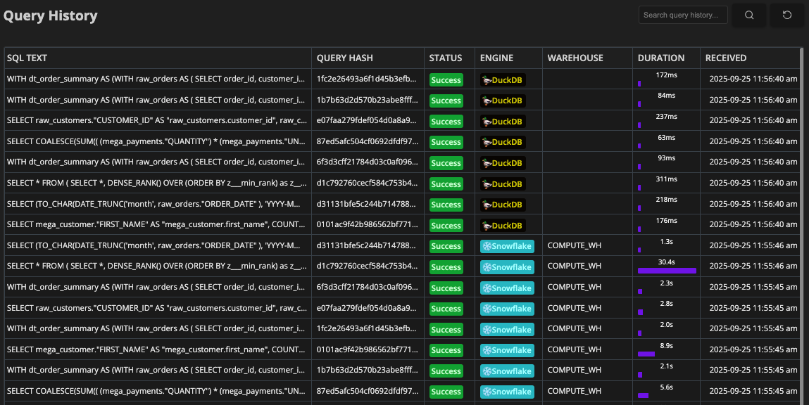
That's why we built Greybeam: to let teams run each query on the engine best suited for it, without having to rewrite queries, replicate data across systems manually, or guess where their workloads will run the fastest. The right engine for the workload isn't a pipe dream anymore, and it can be the difference between a query that runs in minutes and one that runs in seconds.
Snowflake optimization is a never-ending task, but with the right techniques (and the right engine) you can make queries that once took minutes to finish in seconds.
Appendix
Column pruning sample query.
-- If you want to exaggerate this example see below
WITH full_facts AS (
    WITH supplier_bal AS (
        SELECT
            *
        FROM snowflake_sample_data.tpch_sf100.supplier
        WHERE
            s_acctbal > 0
    ),
    items_filtered AS (
        SELECT
            -- uncomment this section to see performance if Snowflake properly column pruned!
            -- l.l_orderkey
            -- , l.l_extendedprice
            -- , l.l_discount
            -- , l.l_shipdate
            -- , l.l_quantity
            -- , l.l_suppkey
            -- , l.l_shipmode
            l.*
        FROM snowflake_sample_data.tpch_sf100.lineitem AS l
        -- replace with lineitem_extended for exaggerated example
        WHERE
            1=1
            AND l.l_partkey IS NOT NULL
            AND l.l_shipmode != 'AIR'
      ),

    items_agg AS (
        SELECT
            l_suppkey
            , COUNT(DISTINCT l.l_orderkey) as num_orders
            , SUM(l.l_extendedprice - l.l_discount) as price
            , SUM(l.l_discount) as total_discount
            , SUM(l.l_discount) / NULLIF(SUM(l.l_extendedprice), 0) as average_disc
            , MIN(l.l_shipdate) as first_shipped
        FROM items_filtered AS l
        GROUP BY 1
        HAVING
            SUM(l.l_extendedprice) > 0
    ),

    shipmodes AS (
        SELECT
            l.l_suppkey
            , l.l_shipmode
            , SUM(l.l_extendedprice - l.l_discount) as revenue
            , SUM(l.l_quantity) as quantity
            , COUNT(DISTINCT (l.l_suppkey)) as supps
        FROM items_filtered AS l
        GROUP BY 1,2
        QUALIFY ROW_NUMBER() OVER (PARTITION BY l.l_suppkey ORDER BY quantity DESC NULLS FIRST, supps DESC NULLS FIRST,  revenue DESC NULLS FIRST) = 1
        )

SELECT
    sb.*
    , s.l_shipmode
    , ia.num_orders
    , ia.price
    , ia.total_discount
    , ia.average_disc
    , ia.price / ia.num_orders AS avg_order_value
    , ia.first_shipped
FROM supplier_bal AS sb
JOIN items_agg AS ia
    ON sb.s_suppkey = ia.l_suppkey
JOIN shipmodes AS s
    ON sb.s_suppkey = s.l_suppkey
)

SELECT
    *
FROM full_facts
;
Exaggerating the example above.
With only 16 seconds, the difference in performance with and without column pruning is only in the 10s of seconds. To exaggerate this example, let's create a temporary table that is an extension of lineitem and re-run our example with this new table.
ALTER WAREHOUSE COMPUTE_WH SET WAREHOUSE_SIZE = 'LARGE';
CREATE TEMPORARY TABLE lineitem_extended AS
    SELECT
    l_orderkey, l_partkey, l_suppkey, l_linenumber, l_quantity, l_extendedprice, l_discount, l_tax, l_returnflag, l_linestatus, l_shipdate, l_commitdate, l_receiptdate, l_shipinstruct, l_shipmode, l_comment,

    l_orderkey AS l_orderkey_1, l_partkey AS l_partkey_1, l_suppkey AS l_suppkey_1, l_linenumber AS l_linenumber_1, l_quantity AS l_quantity_1, l_extendedprice AS l_extendedprice_1, l_discount AS l_discount_1, l_tax AS l_tax_1, l_returnflag AS l_returnflag_1, l_linestatus AS l_linestatus_1, l_shipdate AS l_shipdate_1, l_commitdate AS l_commitdate_1, l_receiptdate AS l_receiptdate_1, l_shipinstruct AS l_shipinstruct_1, l_shipmode AS l_shipmode_1, l_comment AS l_comment_1,

    l_orderkey AS l_orderkey_2, l_partkey AS l_partkey_2, l_suppkey AS l_suppkey_2, l_linenumber AS l_linenumber_2, l_quantity AS l_quantity_2, l_extendedprice AS l_extendedprice_2, l_discount AS l_discount_2, l_tax AS l_tax_2, l_returnflag AS l_returnflag_2, l_linestatus AS l_linestatus_2, l_shipdate AS l_shipdate_2, l_commitdate AS l_commitdate_2, l_receiptdate AS l_receiptdate_2, l_shipinstruct AS l_shipinstruct_2, l_shipmode AS l_shipmode_2, l_comment AS l_comment_2,

    l_orderkey AS l_orderkey_3, l_partkey AS l_partkey_3, l_suppkey AS l_suppkey_3, l_linenumber AS l_linenumber_3, l_quantity AS l_quantity_3, l_extendedprice AS l_extendedprice_3, l_discount AS l_discount_3, l_tax AS l_tax_3, l_returnflag AS l_returnflag_3, l_linestatus AS l_linestatus_3, l_shipdate AS l_shipdate_3, l_commitdate AS l_commitdate_3, l_receiptdate AS l_receiptdate_3, l_shipinstruct AS l_shipinstruct_3, l_shipmode AS l_shipmode_3, l_comment AS l_comment_3,

    l_orderkey AS l_orderkey_4, l_partkey AS l_partkey_4, l_suppkey AS l_suppkey_4, l_linenumber AS l_linenumber_4, l_quantity AS l_quantity_4, l_extendedprice AS l_extendedprice_4, l_discount AS l_discount_4, l_tax AS l_tax_4, l_returnflag AS l_returnflag_4, l_linestatus AS l_linestatus_4, l_shipdate AS l_shipdate_4, l_commitdate AS l_commitdate_4, l_receiptdate AS l_receiptdate_4, l_shipinstruct AS l_shipinstruct_4, l_shipmode AS l_shipmode_4, l_comment AS l_comment_4,

    l_orderkey AS l_orderkey_5, l_partkey AS l_partkey_5, l_suppkey AS l_suppkey_5, l_linenumber AS l_linenumber_5, l_quantity AS l_quantity_5, l_extendedprice AS l_extendedprice_5, l_discount AS l_discount_5, l_tax AS l_tax_5, l_returnflag AS l_returnflag_5, l_linestatus AS l_linestatus_5, l_shipdate AS l_shipdate_5, l_commitdate AS l_commitdate_5, l_receiptdate AS l_receiptdate_5, l_shipinstruct AS l_shipinstruct_5, l_shipmode AS l_shipmode_5, l_comment AS l_comment_5,

    l_orderkey AS l_orderkey_6, l_partkey AS l_partkey_6, l_suppkey AS l_suppkey_6, l_linenumber AS l_linenumber_6, l_quantity AS l_quantity_6, l_extendedprice AS l_extendedprice_6, l_discount AS l_discount_6, l_tax AS l_tax_6, l_returnflag AS l_returnflag_6, l_linestatus AS l_linestatus_6, l_shipdate AS l_shipdate_6, l_commitdate AS l_commitdate_6, l_receiptdate AS l_receiptdate_6, l_shipinstruct AS l_shipinstruct_6, l_shipmode AS l_shipmode_6, l_comment AS l_comment_6
FROM snowflake_sample_data.tpch_sf100.lineitem;
ALTER WAREHOUSE COMPUTE_WH SUSPEND;
ALTER WAREHOUSE COMPUTE_WH SET WAREHOUSE_SIZE = 'XSMALL';
Try this in DuckDB!
Boot up DuckDB 1.4.0 and execute below to see column pruning (or lack thereof) in action!
.timer on
install tpch;
load tpch;
call dbgen(sf=10); -- or use sf=1 depending on your machine
Create a wide table with lineitem
CREATE TEMPORARY TABLE lineitem_extended AS
    SELECT
    l_orderkey, l_partkey, l_suppkey, l_linenumber, l_quantity, l_extendedprice, l_discount, l_tax, l_returnflag, l_linestatus, l_shipdate, l_commitdate, l_receiptdate, l_shipinstruct, l_shipmode, l_comment,

    l_orderkey AS l_orderkey_1, l_partkey AS l_partkey_1, l_suppkey AS l_suppkey_1, l_linenumber AS l_linenumber_1, l_quantity AS l_quantity_1, l_extendedprice AS l_extendedprice_1, l_discount AS l_discount_1, l_tax AS l_tax_1, l_returnflag AS l_returnflag_1, l_linestatus AS l_linestatus_1, l_shipdate AS l_shipdate_1, l_commitdate AS l_commitdate_1, l_receiptdate AS l_receiptdate_1, l_shipinstruct AS l_shipinstruct_1, l_shipmode AS l_shipmode_1, l_comment AS l_comment_1,

    l_orderkey AS l_orderkey_2, l_partkey AS l_partkey_2, l_suppkey AS l_suppkey_2, l_linenumber AS l_linenumber_2, l_quantity AS l_quantity_2, l_extendedprice AS l_extendedprice_2, l_discount AS l_discount_2, l_tax AS l_tax_2, l_returnflag AS l_returnflag_2, l_linestatus AS l_linestatus_2, l_shipdate AS l_shipdate_2, l_commitdate AS l_commitdate_2, l_receiptdate AS l_receiptdate_2, l_shipinstruct AS l_shipinstruct_2, l_shipmode AS l_shipmode_2, l_comment AS l_comment_2,

    l_orderkey AS l_orderkey_3, l_partkey AS l_partkey_3, l_suppkey AS l_suppkey_3, l_linenumber AS l_linenumber_3, l_quantity AS l_quantity_3, l_extendedprice AS l_extendedprice_3, l_discount AS l_discount_3, l_tax AS l_tax_3, l_returnflag AS l_returnflag_3, l_linestatus AS l_linestatus_3, l_shipdate AS l_shipdate_3, l_commitdate AS l_commitdate_3, l_receiptdate AS l_receiptdate_3, l_shipinstruct AS l_shipinstruct_3, l_shipmode AS l_shipmode_3, l_comment AS l_comment_3,

    -- Uncomment below if you want an even more stark example!
    -- l_orderkey AS l_orderkey_4, l_partkey AS l_partkey_4, l_suppkey AS l_suppkey_4, l_linenumber AS l_linenumber_4, l_quantity AS l_quantity_4, l_extendedprice AS l_extendedprice_4, l_discount AS l_discount_4, l_tax AS l_tax_4, l_returnflag AS l_returnflag_4, l_linestatus AS l_linestatus_4, l_shipdate AS l_shipdate_4, l_commitdate AS l_commitdate_4, l_receiptdate AS l_receiptdate_4, l_shipinstruct AS l_shipinstruct_4, l_shipmode AS l_shipmode_4, l_comment AS l_comment_4,

    -- l_orderkey AS l_orderkey_5, l_partkey AS l_partkey_5, l_suppkey AS l_suppkey_5, l_linenumber AS l_linenumber_5, l_quantity AS l_quantity_5, l_extendedprice AS l_extendedprice_5, l_discount AS l_discount_5, l_tax AS l_tax_5, l_returnflag AS l_returnflag_5, l_linestatus AS l_linestatus_5, l_shipdate AS l_shipdate_5, l_commitdate AS l_commitdate_5, l_receiptdate AS l_receiptdate_5, l_shipinstruct AS l_shipinstruct_5, l_shipmode AS l_shipmode_5, l_comment AS l_comment_5,

    -- l_orderkey AS l_orderkey_6, l_partkey AS l_partkey_6, l_suppkey AS l_suppkey_6, l_linenumber AS l_linenumber_6, l_quantity AS l_quantity_6, l_extendedprice AS l_extendedprice_6, l_discount AS l_discount_6, l_tax AS l_tax_6, l_returnflag AS l_returnflag_6, l_linestatus AS l_linestatus_6, l_shipdate AS l_shipdate_6, l_commitdate AS l_commitdate_6, l_receiptdate AS l_receiptdate_6, l_shipinstruct AS l_shipinstruct_6, l_shipmode AS l_shipmode_6, l_comment AS l_comment_6
FROM lineitem;
Run the query!
WITH supplier_bal AS (
        SELECT
            *
        FROM supplier
        WHERE
            s_acctbal > 0
    ),
    items_filtered AS (
        SELECT
            -- uncomment this section to see the performance difference!
            -- l.l_orderkey
            -- , l.l_extendedprice
            -- , l.l_discount
            -- , l.l_shipdate
            -- , l.l_quantity
            -- , l.l_suppkey
            -- , l.l_shipmode
            l.*
        FROM lineitem_extended AS l
        WHERE
            1=1
            AND l.l_partkey IS NOT NULL
            AND l.l_shipmode != 'AIR'
      ),

    items_agg AS (
        SELECT
            l_suppkey
            , COUNT(DISTINCT l.l_orderkey) as num_orders
            , SUM(l.l_extendedprice - l.l_discount) as price
            , SUM(l.l_discount) as total_discount
            , SUM(l.l_discount) / NULLIF(SUM(l.l_extendedprice), 0) as average_disc
            , MIN(l.l_shipdate) as first_shipped
        FROM items_filtered AS l
        GROUP BY 1
        HAVING
            SUM(l.l_extendedprice) > 0
    ),

    shipmodes AS (
        SELECT
            l.l_suppkey
            , l.l_shipmode
            , SUM(l.l_extendedprice - l.l_discount) as revenue
            , SUM(l.l_quantity) as quantity
            , COUNT(DISTINCT (l.l_suppkey)) as supps
        FROM items_filtered AS l
        GROUP BY 1,2
        QUALIFY ROW_NUMBER() OVER (PARTITION BY l.l_suppkey ORDER BY quantity DESC NULLS FIRST, supps DESC NULLS FIRST,  revenue DESC NULLS FIRST) = 1
        )

SELECT
    sb.*
    , s.l_shipmode
    , ia.num_orders
    , ia.price
    , ia.total_discount
    , ia.average_disc
    , ia.price / ia.num_orders AS avg_order_value
    , ia.first_shipped
FROM supplier_bal AS sb
JOIN items_agg AS ia
    ON sb.s_suppkey = ia.l_suppkey
JOIN shipmodes AS s
    ON sb.s_suppkey = s.l_suppkey
;

Comments ()