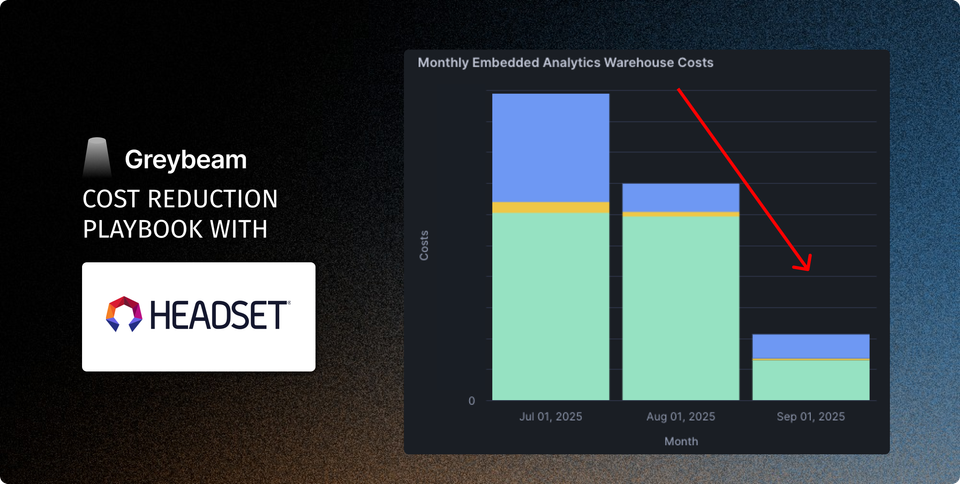
How Headset Cut Snowflake BI Costs by 83% While Supporting 2,500+ Users

In this playbook, we share Headset's journey and the blueprint you can use to build a data stack that keeps performance high and costs low, even at scale.

Results at a Glance

• 83% reduction in Snowflake costs to serve embedded analytics
• No migration or SQL rewrites
• Savings realized instantly after rollout

Headset is the leading cannabis data and analytics platform trusted by thousands of retailers, producers, and brands across the U.S. and Canada, providing real-time visibility into sales, inventory, staffing, and supply-chain.

Featuring

As CTO, Scott Vickers leads the analytics strategy at Headset, ensuring the platform delivers consistent performance at scale while keeping Snowflake costs under control.

The good news is that you can learn from Scott's playbook on how he reduced Snowflake embedded analytics spend by 83% at Headset, all while keeping performance fast and reliable.

Let's dive in.

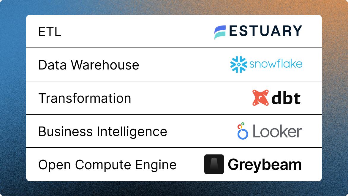
The Stack

The Ingestion Journey

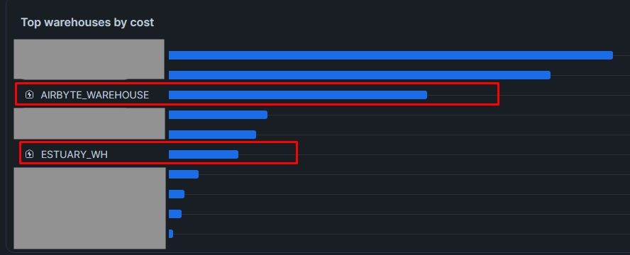
Headset had relied on Fivetran for years, but an unexpected pricing change meant their ingestion bill was about to jump by more than 50%. To keep costs in check, Scott moved the team to Airbyte, which immediately lowered vendor spend.

However, within weeks, ingestion compute had increased by 50%. Airbyte’s scan-heavy, multi-step loading pattern shifted the cost burden from the vendor onto Snowflake (at the time of writing, this has been addressed by the Airbyte team here). Scott realized that to truly lower costs, he needed a tool that was both economical and engineered to load data efficiently.

That’s where Estuary came in.

Estuary streams incremental changes via Snowpipe or loads micro-batches using highly optimized merge operations that avoid full-table scans. Because it processes only true deltas, Snowflake handles dramatically less work on every load.

The impact was immediate:

Optimizing Snowflake

Over the years, Scott used multiple techniques to refine and refactor the core of Headset’s analytics models making them faster, leaner, and more predictable.

Breaking Up One Big Tables

Queries against a single monolithic model slowed down dashboard loads and forced Snowflake to do more work than necessary.

Scott refactored Headset's one-big-tables into purpose-built models tailored to individual dashboards and workflows. The result was faster build times and reduced downstream compute footprint, since every model only processed the data it truly needed.

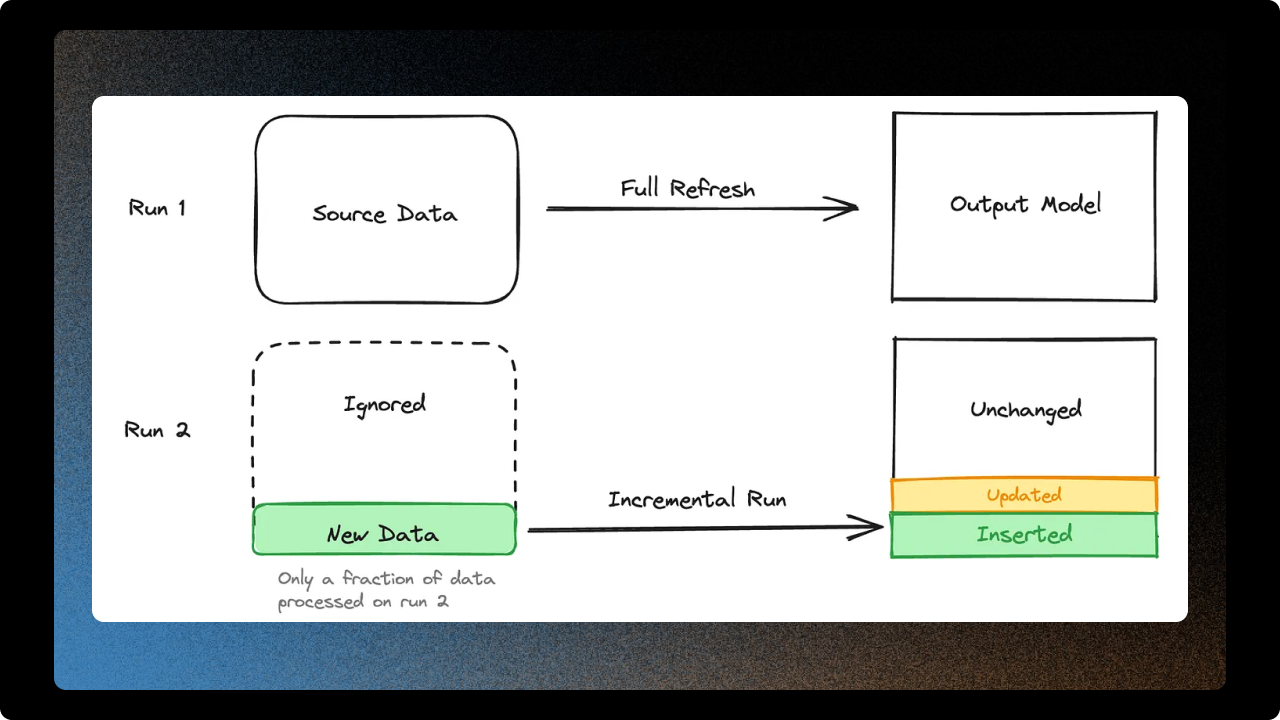
Incrementalizing and Viewifying Materializations

A big part of controlling Snowflake costs is choosing the right materialization strategy. Lightweight transforms don’t always need to be tables. If a model is just a simple filter, rename, or join on already well-modeled data and it isn’t hit constantly by dashboards, it’s usually cheaper to make it a view because it doesn't need to be rebuilt.

For heavier models, the opposite default applies: assume they should be incremental. Rebuilding an entire multi-terabyte table wastes compute when only today’s or the last hour’s data has changed.

Incremental models aren’t always cheaper; they can backfire in scenarios like:

• Models with window functions that require historical data.
• A significant portion of the table changes on each load.
• Poor partition pruning.
• Small tables: the overhead of incremental logic can cost more than reloading the table.
• Complex incremental logic: merge operations can get expensive if not properly pruned.

Per-Model Warehouse Sizing

Teams tend to fall into the trap of using the warehouse size that can accommodate their largest models, this means tables and tests that could otherwise use an XS end up building on a larger warehouse.

Scott took a granular approach and wrote a dbt macro to adjust the warehouse size depending on the model and materialization strategy.

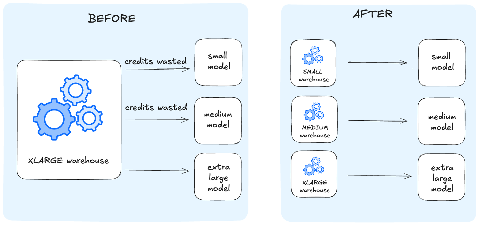
By sizing compute to the real workload of each model, Scott kept his dbt build performant without overspending.

{{
    config(
        materialized='table',
        tags = 'hourly'
    )
}}

{{ get_warehouse_size(full_refresh_size='large', incremental_size='small') }}

-- rest of dbt model here

Reducing Unnecessary Runs

Adjusting the dbt schedule is one of the simplest and most overlooked ways to drastically reduce Snowflake costs. If a model that runs every hour can instead run every two hours, you’ve instantly reduced its compute cost by 50% without touching a single line of SQL. Scott applied this lens across all his pipelines, asking a basic question for every model: Does this really need to refresh this often?

By distinguishing which models needed real-time freshness and which ones didn’t, he was able to meet product SLAs while keeping costs to a minimum. After all, very few dashboards need a full rebuild at 3 a.m. on a Saturday.

Optimizing Embedded Analytics

Balancing performance and cost is far trickier in customer-facing embedded analytics than in traditional BI. In a dashboard, most users will tolerate seconds of load time. Inside a customer-facing product, those same few seconds can feel dreadfully slow.

Right-sizing Your Warehouse

Customer-facing embedded analytics leads to unpredictable traffic patterns. A quiet period can instantly turn into a surge when dozens of users load dashboards at once. On a Snowflake Standard account, this is especially challenging because horizontal scaling isn’t available, you can’t spin up multiple clusters to handle concurrency. The only lever you have is warehouse size, and running a large warehouse becomes expensive fast.

To address this, Scott built a script that monitors recent query activity in a rolling window and automatically adjusts warehouse size based on real load. During peak hours, the warehouse scales up to provide consistent performance for over 2500 users. During off-hours, it scales back down so that a late-night dashboard refresh uses an XS.

We've attached Scott's script at the end of this blog.

Using the Right Engine to Serve Embedded Analytics

Snowflake is excellent for many things, but it was never designed to affordably serve queries to over 2500 users with sporadic usage patterns.

At some point, the question wasn’t “How do we optimize Snowflake further?” but rather “Is Snowflake the right tool for this part of the workload?”

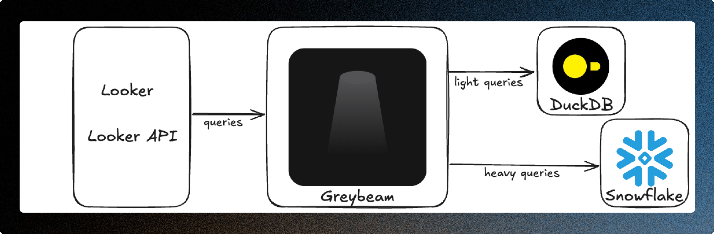
That’s where Greybeam changed everything. Instead of forcing every Looker query to run on Snowflake, Greybeam provides fully managed DuckDB clusters and automatically translates and routes eligible queries to DuckDB, without any migration.

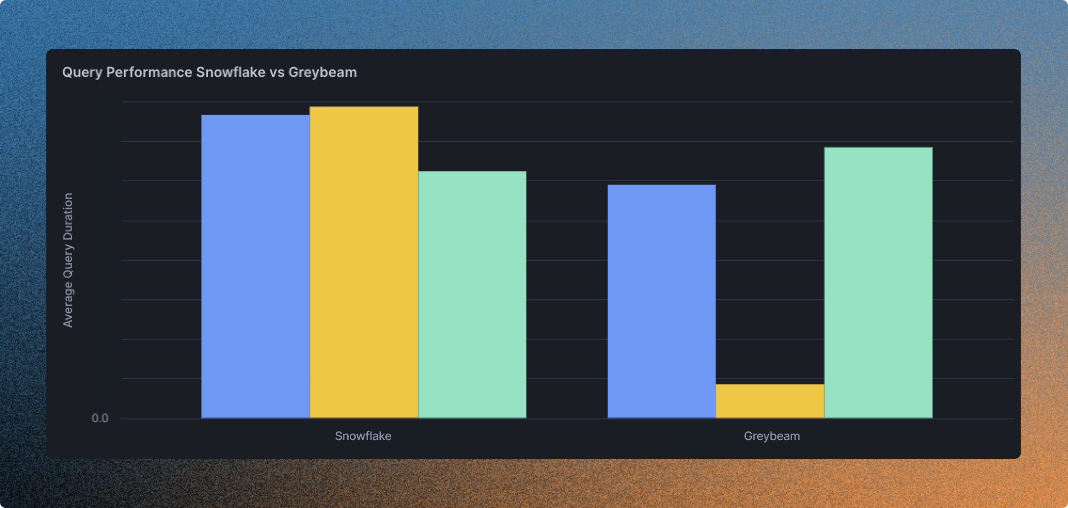
The savings were immediate with 94% of queries routed to DuckDB and an average drop of 83% in Snowflake costs. What had once been one of Headset’s largest Snowflake expenses became one of the smallest, all while keeping dashboards fast and reliable for users.

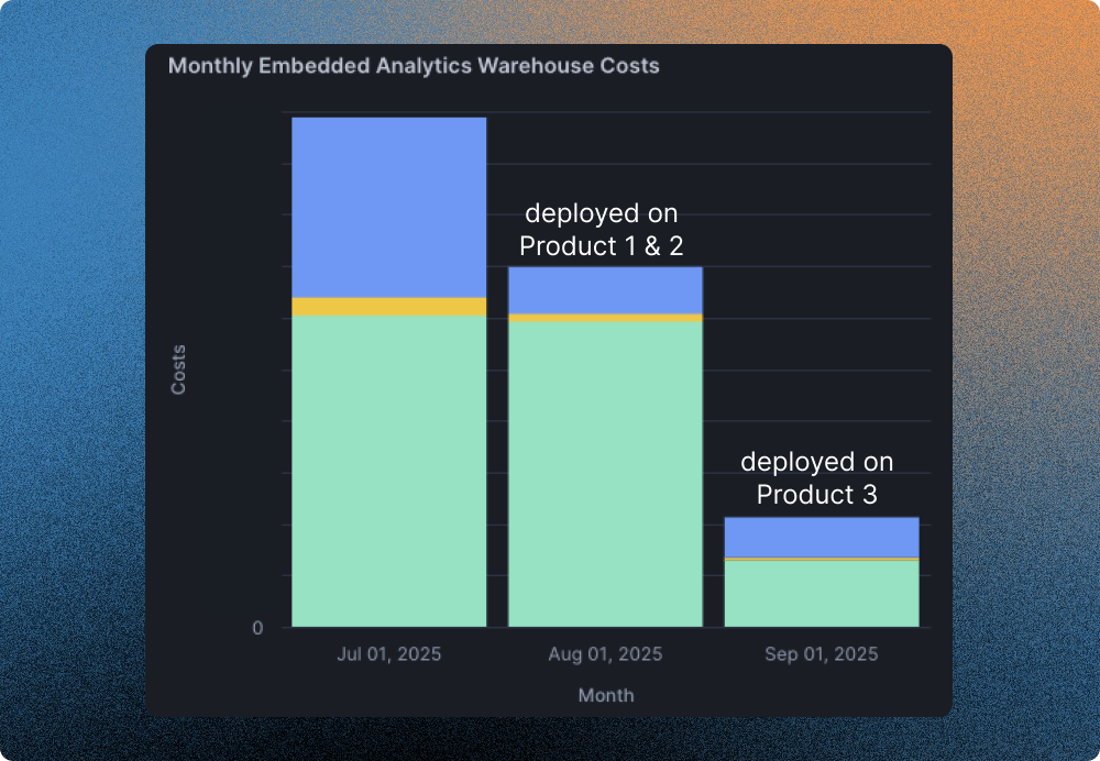
Greybeam didn’t replace Snowflake; it complemented it. Scott kept the same great Snowflake developer experience, while offloading a majority of traffic to DuckDB, a far more cost-effective engine. For Scott, it was the piece that finally aligned performance, scale, and cost.

What's Next?

For Headset, the future is a data stack where ingestion, transformations, and analytics each run on the engine best suited for the job. And with Greybeam, Scott sees a path to making that architecture both high-performing and significantly more cost-effective.

The next major opportunity is bringing the same cost-efficiency to the transformation layer. Greybeam is actively developing support for offloading dbt model builds onto more efficient compute.

As Greybeam expands into the transformation layer, teams like Headset will have a path to reduce Snowflake costs end-to-end across ingestion, transformations, and embedded analytics, all while preserving the Snowflake developer experience their teams rely on.

Scott's warehouse script.

CREATE OR REPLACE PROCEDURE adjust_wh_size_by_qps_js()
  RETURNS STRING
  LANGUAGE JAVASCRIPT
  EXECUTE AS CALLER
AS
$$
  const warehouse = '<warehouse_name>';    // ← your warehouse name (case‑sensitive)
  const threshold = 150;           // ← queries in last 10 min to trigger MEDIUM

  // 1) Count queries in the past 10 minutes
  const cntStmt = snowflake.createStatement({
    sqlText: `
      SELECT COUNT(*) AS Q_CNT
        FROM snowflake.account_usage.query_history
       WHERE warehouse_name = ?
         AND start_time > DATEADD(minute, -10, CURRENT_TIMESTAMP())
         AND start_time <= CURRENT_TIMESTAMP()
    `,
    binds: [warehouse]
  });
  const cntRes = cntStmt.execute();
  cntRes.next();
  const qCnt = cntRes.getColumnValue('Q_CNT');

  // 2) Decide target size
  const newSize = (qCnt >= threshold) ? 'MEDIUM' : 'X-SMALL';

  // 3) Fetch current size via SHOW
  const showStmt = snowflake.createStatement({
    sqlText: `SHOW WAREHOUSES LIKE ?`,
    binds: [warehouse]
  });
  const showRes = showStmt.execute();
  showRes.next();
  // "size" column holds the warehouse size
  const currentSize = showRes.getColumnValue('size').toUpperCase();


  snowflake.createStatement({
    sqlText: `
      INSERT INTO wh_size_history(warehouse, old_size, new_size, q_cnt)
      VALUES(?, ?, ?, ?)
    `,
    binds: [warehouse, currentSize, newSize, qCnt]
  }).execute();
  

  // 4) Only ALTER if it differs, and return accordingly
  if (currentSize !== newSize) {
    snowflake.createStatement({
      sqlText: `ALTER WAREHOUSE ${warehouse} SET WAREHOUSE_SIZE = "${newSize}"`
    }).execute();
    return `Ran ${qCnt} queries → resized from ${currentSize} to ${newSize}`;
  } else {
    return `Ran ${qCnt} queries → kept at ${currentSize}`;
  }
$$;

Written with 🛩️.